Automated Bedrock Channel Width Extraction

Problem & Background

Bedrock river width is an essential geometric parameter relevant to understanding flood hazards and gauging station rating curves, and is critical to stream power incision models and many other landscape evolution models. Obtaining bedorck river width measurements, however, typically requires extensive field campaigns that take place in rugged and steep topography where river access is often physically challenging. Although previous work has turned to obtaining these measurements from satellite imagery, these data present a snapshot in time (e.g. not necessarily under a particular or desired discharge scenario), are typically limited to rivers >10-30 m wide due to image resolution, and are physically restricted to areas devoid of vegetation. For these reasons, information of bedrock channel width is generally data limited, and the factors impacting bedrock channel width remain poorly understood. Due to these limitations, researchers often use a width-scaling relationship based on alluvial rivers, which form and change differently than bedrock rivers.

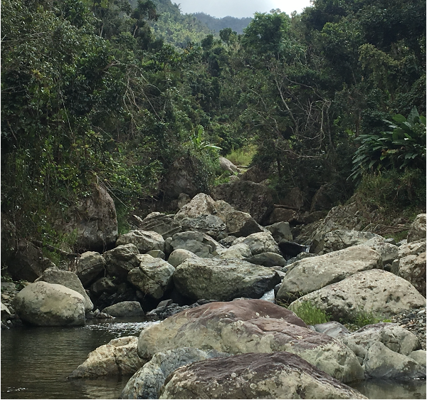
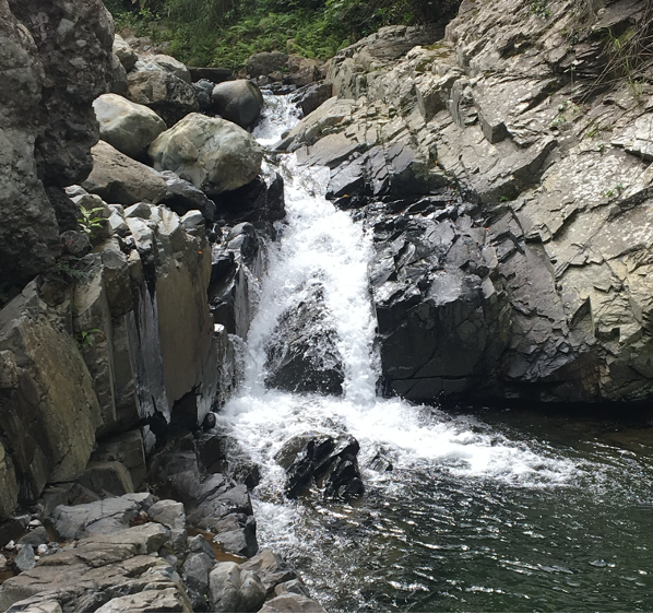
In this project, I develop a new method to remotely obtain bedrock channel width at a desired river discharge. Analysis of rivers in Puerto Rico show that modeling results generally fall within measurement error of verified field measurements from USGS gauging stations used to determine rating curves of streamflow gauges. As a result, this method proves to work at estimating bedrock channel width on a large scale, remotely, and efficiently at equal discharge scenarios, providing an avenue for researchers and scientists to glean more measurements remotely without the need of expensive field campaigns.

Method to address problem

General Overview

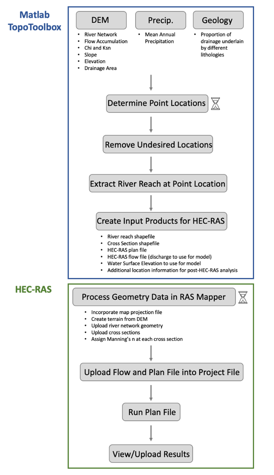
The cornerstone of this analysis is the use of a high-resolution digital elevation model (DEM). Over the past few years, there has been an increased effort to acquire high-resolution DEMs through LiDAR flight campaigns. The U.S. Geological Survey’s 3D Elevation Program (3DEP), for example, will provide free access to high-resolution LiDAR across the continental United States within the next year. With this in mind, this method will be able to be applied to nearly any location in the United States.

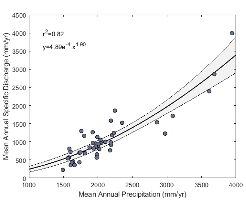
A first step of the project is to use the DEM to learn more about an area and determine sampling locations. One challenge of this analysis is to discern discharge across each sampling location at a comparible return interval (e.g. each location’s 1-year RI discharge is different, based on upstream watershed area). As a result, we first model the relationship between known locations (e.g. USGS gauging stations) and the precipitation record. We then derive the specific precipitation (e.g. precipitation total per square meter), and combine this value with each location’s upstream drainage area to derive the estimated discharge at a given location.

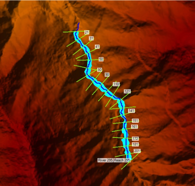
To perform the model simulation, we need to create shapefiles of the river at each sampling point, and model channel width across the desired stream reach. Although it is possible to manually do this, doing so is inefficient at a large scale. As a result, we derive a channel segment of desired length at each location, and define cross sections perpendicular to the river at a desired increment.

Once these channel segments are created, we import the data and run the simulations in the HEC-RAS modeling software. HEC-RAS is a freely-available platform created by the U.S. Army Corps of Engineers, and used widely throughout the environmentl consulting industry. Once modeled, data outputs from the simulations can be used to efficiently evaluate trends in channel width across different bedrock types and environments.

In-Depth Method Overview

Follow the mark-up document below to step through the code of the process described above!

%Define files
selpath='Add path here';
%Create a new folder for analyzed watershed
newfolder=append('selpath,'\WS_Name');
mkdir (newfolder);
StreamFolder=append(newfolder,'\Streams');
XSectFolder=append(newfolder,'\CrossSections');
DataFolder=append(newfolder,'\Data');
mkdir (StreamFolder);
mkdir(XSectFolder);
mkdir(DataFolder);

%Load DEM
DEM_Loc=append(selpath,'\DEM_',string(WS),'.tif')
DEM=GRIDobj (DEM_Loc)

%Fill in all sinks in the LiDAR dataset and take out all blank/nan values
DEM.Z(DEM.Z <=0)=nan;
DEMf= fillsinks(DEM);
DEMf= inpaintnans(DEMf);

%Load Geologic Map
GEOL_Loc=append(selpath,'\GEOL_',str(WS),'.tif');
GEOL=GRIDobj(GEOL_Loc);

%Load Precipitation map
PRECIP_Loc=append(selpath,'\PRECIP_',string(WS),.tif');
PRECIP=GRIDobj(GEOL_Loc);

%Derive flow accumulation and river network
FD= FLOWobj(DEMf);
cellsize=1e6;
A= flowacc(FD).*DEMf.cellsize^2;
crita=1e5;
S= STREAMobj(FD,'minarea',crita./DEM.cellsize^2);
S=removeshortstreams(S,100);
mn=0.45; %set concavity index.
Ao=1; %set reference drainage area you would like to use,
here we use 1 km^2
smoWin=500; %set smoothing window for Chi analysis.

%Make sure that the DEM, Geology, and precipitation files l
ine up with one another
[DEMf,GEOL]=largest_overlapping_extent(DEM,GEOL);
[DEMf,PRECIP]=largest_overlapping_extent(DEM,PRECIP)

%View side-by-side image
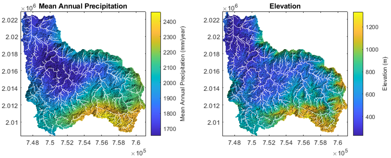
figure()
subplot(1,2,1)
imageschs(PRECIP); %precipitation
hold on;
imageschs(DEMf); %DEM (w/ filled sinks)

%Determine unique geologic formations in your area of analysis.
Fmn=GEOL.Z(:);
Fmn(isnan(Fmn))=[];
Geol_Fmn=unique(Fmn);

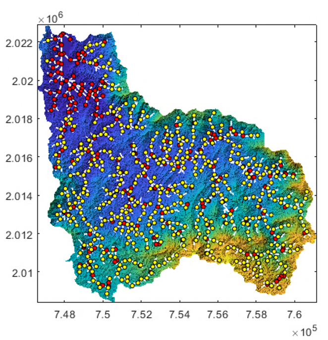
%Select all locations based on a defined drainage area
D_vect=105:500:max(S.distance)-105; Here we select
points every 500 meters along the stream network.

[d_mat]= XS_Selection_Info(DEMf,GEOL,FD,ksnGrid,chiGrid,A,S, D_vect, PRECIP)
%this is a sub-routine that I have developed to create a table tha
 includes attributes including: long/lat locations, point index,
 drainage area at point, average precipitation at the point, elevation
 at point, average upstream drainage area elevation and steepness,
  as well as the proportion of each unique geologic unit in each
   upstream watershed.

%Change the matrix to a table
T-array2table(d_mat);

%Remove all location points that are in bodies of water
(we want to focus on rivers after all, not reservoir/lakes!)
E=sum(ismember(T.Properties.VariableNames.'Geol_5'));
if E>0
    L=find(T.Geol_at_ix==5);
    T(L,:)=[];
end

%The HEC-RAS program (used later) does not work if any river
segments overlap. Make sure that we don't have overlapping
river segments (e.g. points within ~200m from e/o), and
remove if we do.
for i=1:length(T.utm_x)
    idx_check=[];
    dist=zeros(length(T.utm)x)-i,1);
    for j=i+1:length(T.utm_x)
        idx_check=[];
        %get distance between initial point and rest of points
        dist(j-i,1)=sqrt(((T.utm_x(j)-T.utm_x(i))^2)+((T.ut_y(j)-T.utm_y(i))^2));
    end
    idx_check=find(dist<=210);;
    idx_check=idx_check+i;
end

%remove the points you extracted in the previous step.
T(idx_check,:)[];

%In another module, we have fit the precipiation and discharge
data at each USGS stream gauge location to a model. During
this step, we derived the model paramters.

%Here we implement the model parameters at each sampling
location to derive specific discharge at each location.
look_up=T.avg_precip_ix;
mdl_yhat=mdl_power_b.*mdl_x.^mdl_power_m;
T.Qsp_fit=interp1(mdl_x,mdl_yhat,lookup,'nearest');

%Determine the desired spacing of each cross section of your shapefile.
XS_space=10; %here we designate a 10m spacing.
[Output]=XS_Creator(S,DEMf,GEOL,Index_Table, XS_space, SX_width);
%here I have created a function that automatically creates
stream shapefiles at each location, as well as cross sections
spaced 10m apart.

%Once the shapefiles have been created, we can extract discharge,
 as well as the estimated downstream water elevation--two parameters
 that are required for the HEC-RAS modeling software.

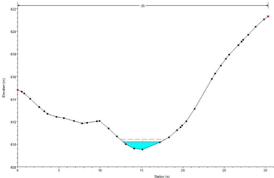
Once created, all of the stream shapefiles are uploaded into HEC-RAS and simulations are performed for your given discharge scenario. From the model runs (see figure below), we can extract the wetted channel width at each cross section. These data can be evaluated further to derive the average channel width at a given discharge at each location.

Method Verification

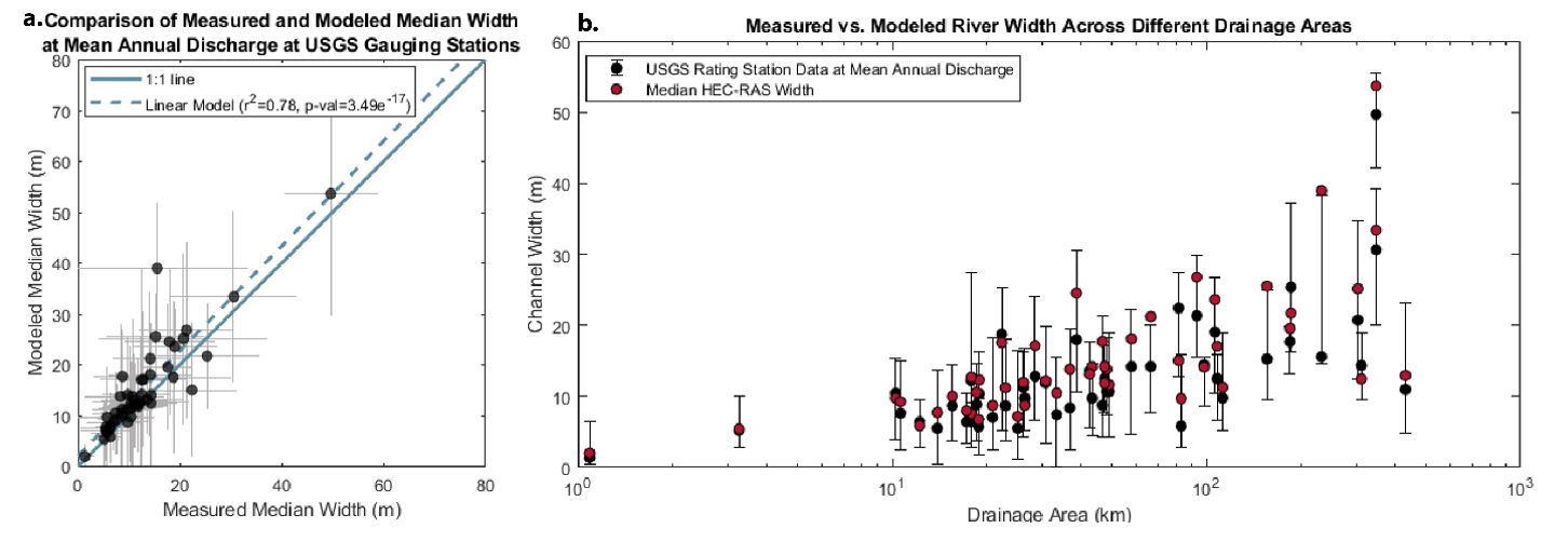
A comparison between modeled HEC-RAS width values in relation to USGS field measurements collected at comparable discharge values (Mean Annual Discharge) show that the method does a good job at predicting channel width. Most modeled width measurements (including error) fall on the 1:1 line (Figure a), indicating that the model generally does a good job at predicting channel width measurements across different locations at the Mean Annual Discharge.

In addition, I compared the modeled HEC-RAS width values in relation to USGS gauging station field measurements. Figure b shows the modeled and measured channel width at comparable discharge values (Mean Annual Discharge) in relation to drainage area. Error bars indicate the maximum and minimum USGS field measurement values at each station. Most HEC-RAS width measurements fall within the variability in USGS field measurements collected at a comparable discharge across a wide span of drainage areas.

For more details about this project, read the paper titled [New remote method to systematically extract bedrock channel width of small catchments across large spatial scales using high-resolution digital elevation models](/publications)